The challenge of perceiving the world starts with the ability of our brain to understand and interpret what is being focused on to our retinas by our eyes. How do we go from a static, flat and overly ambiguous 2D retinal image (the image that each eye sees) to the meaningful perception of our world?

How do we get from a series of points and lines to a meaningful visual perception?
To date, there have been many proposed models on how we get from the basic 2D retinal image to our 3D visual perceptions. The main theories of this are described below.
Top-Down Processing (Top)
Top-down processing is the use of high level cortical processing to form a visual perception. In lay terms, this means that we use what we already know about the world to influence what we perceive. Evidence to support this theory comes in the shape of an experiment conducted by vision scientist Irving Biedermann in 1981.

The Goodrich Telephone Illustration - showing visual violations of size,
support and probability (Image: Biedermann 1981)
In his experiment, Biedermann presented subjects with a visual scene and asked them to locate a certain object, which in this case was a telephone. He found that more errors were made in the perception of the image where objects in a scene were in, what he called, physical violation. Such physical violations include the lack of support (a telephone floating in mid-air), position (the telephone appearing on a building), interposition (being able to see the background through the telephone), size (where the telephone's size was out of expected proportion to the scene and probability (the telephone appearing in an unexpected place, such as in a car or in a kitchen).
This shows that the observer's knowledge of the properties of fire hydrants influenced their perception of the scene. More information can be found on this experiement in his paper, accessible here: Biedermann 1981.
Bottom-Up Processing (Top)
Bottom-up processing is where the image is analysed as retinal image parts and combined into a perception. This is a low-level processing theory and works as this: an object is seen in the centre of the observer's vision and the sight of the object and all of its visual stimulus are transmitted from the retina and to the visual cortex (the part of the brain that processes visual input from the eyes). The direction of this visual input is in one direction.

The image environment provides us enough information to see the lady's size, shape and how
far away she is, even though we may not have seen a lady like this before (Image/Pixabay)
The psychologist Eleanor Jack Gibson strongly supported the hypothesis that vision is bottom-up and declared a "what you see is what you get" approach that visual perception is a direct phenomenon. She explained that the environment provides sufficient information related to the stimulus observed (for example shape, size, colour and distance away) that we can perceive the stimulus confidently and without prior experience or knowledge of it. Apply this to the photograph above. More on this can be read on the Simply Pscyhology website.
This hypothesis is also supported by motion parallax. When on a fast moving vehicle, such as a car or train and we look out of the window, we perceive the objects that are closer to us to move by much faster than the objects that are much further away. Therefore we are able to form a perception of the distance between us and the objects passing us by, based by the speed they pass. An example of this can be seen in the video clip below.
A video showing parallax motion. Note how the field details of the puddles pass by quickly, allowing us to perceive them as closer, but the trees further back move by us much more slowly, allowing us to perceive the structure as much further away. Video/eyesonjason
It is likely that there are elements of both top-down processing and bottom-up processing in our visual perception of the world. The next few sections look at slightly more complex models of image analysis.
Treisman's Feature Integration Theory (Top)
In 1980, vision scientists Anne Treisman and Garry Gelade developed the feature-integration theory. The feature-integration theory has become one of the most influential models of visual perception.
Their theory states that attention must be directed to each stimulus in series to characterise and distinguish between the objects presented to our vision. The objects are then separated and sorted into primitive features (such as texture and colour) before being integrated into a whole perception. This process occurs in several stages:
")
A diagram showing the process of object recognition through Treisman's Feature Integration Theory.
Stage 1:
The first stage is the pre-attentive stage (i.e. the stage that occurs in early perceptual processing and before we become conscious of the object). In this stage, the retinal image is broken down into primitives (also known as pre-attentives), which are the elementary components of the retinal image. These primitives include colour, orientation, texture and movement.
Stage 2:
The second stage is the focused-attention stage. In this stage, all of the primitives/pre-attentives are recombined to form a whole perception of the object. We are conscious and aware of the object at this stage.
Stage 3:
The final stage is where top-down processing occurs and our brain compares the recombined perception of the image. These features are then stored in our memory banks as an object file. If we are familiar with the object, top-down processing allows for links to be made between the object and prior knowledge or experience, which leads to the object being identified.
There are two types of visual searching tasks; the "feature search" and the "conjunction search". These feature searches can occur fast (within 250 ms) whilst looking for primitives of one feature (i.e. shape/colour/orientation etc.). The primitives that are different tend to make themselves stand out from the rest. On the other hand, conjunction searches occur when the primitives have two or more features to distinguish from and requires effort from the conscious brain. Therefore conjunction searches are more demanding and can take longer to perform. This is demonstrated in the diagram on the right, where the top two tasks are feature searches and the bottom task is the conjunction search. Further information on this can be found in Treismann and Gelade's paper.

The Marr-Hildreth Computational Model (Top)
The Marr-Hildreth computational model, put forward by David Marr and Ellen C Hildreth, uses mathematical operators to explain the process of vision. The basic process involves the retinal image being analysed for primitives, which forms a raw primal sketch. These primitives are then grouped together and processed to form a 2½ dimensional sketch. The brain then is able to form a 3 dimensional perception of the object being seen.

The process involved in the Marr-Hildreth Computational Model
This occurs in stages, as outlined in the diagram above. The first step is to identify edges and primitives. Every image is made up of changes in luminance over space that, when analysed, will form a luminance profile. These luminance profiles formed from images are complex and formed of lots of peaks and troughs. These peaks and troughs are caused by the edges found in the image. Some peaks and troughs are formed by variations in the surface texture, shading, lighting and other imperfections in the surface. The brain therefore has to correctly identify the important edges in changing luminances.
Edges and Edge Detection (Top)

How edges are detected through luminance profiles and their first derivative
An edge is defined as a point where there is a sudden change in luminance over space. In order to detect an object, the brain must be able to extract these edges from complicated luminance profiles. To identify the parts of the luminance profile where the luminance is changing most steeply across space, the gradient (dl/dx) of the luminance profile must be considered. This provides us with the first derivative of the profile (i.e. the information from the profile where the luminance changes occur the most). This is summarised in the diagram to the left.
In some cases the edges may not be sharp, so there will not be a sharp peak on the first derivative profile. Therefore a second derivative can be obtained and the point where the second derivative crosses the x-axis can be taken as the edge. These are known as zero crossings. An example of this can be seen in the diagram below.

A gradual changing luminance profile, with its first and second derivatives
Difficulties with the Marr-Hildreth Model (Top)
There are two main difficulties with this model:
1) Retinal images are two dimensional and not one dimensional. This means you cannot just look for edges in one direction (such as left to right). If the zero-crossings were only taken from the x-axis, then the horizontal edges will be missed and the image will be incomplete. With this in mind, you would need to get the second derivatives in both the horizontal and vertical axes and extract the zero-crossing values for them both. The sum of the vertical and horizontal second derivatives is known as the Laplacian Operator, which will be expanded upon later.
2) The second problem with the Marr-Hildreth Model is the presence of noise. Luminance profiles tend to suffer from a noisy signal generated from fluctuations in illumination level and, in the instance of biological vision, neural noise (the fluctuations caused by random excitations of the neurons in the nervous system). Unfortunately for the model, these fluctuations are amplified and exaggerated by the derivative operations.
More information on the Marr-Hildreth Model can be seen in their paper, available by clicking the link.
This is where smoothing comes in useful. Smoothing involves averaging together the adjacent inputs of pixels (computer) or photoreceptors (biological eye) and this averaging produces a much smoother luminance profile. In the human eye, this smoothing comes from the retinal ganglion cells averaging the input of adjacent photoreceptor cells.

The effect of smoothing on an otherwise noisy luminance profile
Marr and Hildreth used Gaussian smoothing, which weights the averaging of pixels to the bell-shaped Gaussian function. Essentially this means the averaging weights heavily the effect of the photoreceptors that occur most centrally and weights lightly the photoreceptors that are further in the periphery of the area averaged. This area averaged is known as the receptive field, which will be covered in more detail in another article in the future.

The effect of smoothing on an otherwise noisy luminance profile. (Image/eyesonjason)
The smoothing was then implemented with the Laplacian operator, to produce the Laplacian of Gaussian operator (from here on in, the LoG operator). The LoG filters out edges and finds the zero-crossings horizontally and vertically in the Gaussian-smoothed image. An example of the end result of the LoG operator can be seen in the picture to the left
The LoG operators also have different sizes of which they operate (i.e. they only detect details of certain sizes). This further matches to the way the eyes have receptive fields. These LoG operators have circular receptive fields to allow the operator to detect edges in all orientations (not just in one direction like the gradient method described earlier). The size of the LoG operator determines the size of the details picked up and in order to detect all the information from an image a range of different sized LoG operators will be required.

Different sized LoG operators have different applications
Each sized filter extracts the candidate edges for that filter and each edge can only be considered a true edge if it is in a similar position and in similar orientation to at least two filters of adjacent sizes. Anything else that is detected, but does not fit this criteria, is considered as noise and thus ignored.
Physiological Evidence for the Marr-Hilldreth Model (Top)
This model has evidence that supports it - coming directly from ourt knowledge on how the human eye works. The two main supporting pieces of evidence are:
1) The numerous different-sized LoG operators fit in well with the evidence of the multiple spatial frequency channels in the visual system. We have different sized receptive fields for the retinal ganglion cells within our eyes, all sensitive to different spatial frequencies. This matches with the multiple sized forms of the LoG operators that are sensitive to different levels of detail.

The spatial frequency function
Two scientific studies can help prove this. The first study, from Blakemore and Campbell in 1969, show that adapting an eye to a sine wave of 6 cycles per degree, there is a reduction in sensitivity to that spatial frequency only. This shows that different spatial frequency channels exist.
The second study, by Maffei and Fiorentini 1973, showed that activity measurements of simple cortical cells differed in response to different spatial frequencies. The tuning curve of each of the tested cortical cells were recorded with different gratings, which were moved over their receptive fields. these channels correspond to channels that underlie the spatial sensitivity function (diagram to the left).
2) The second reason is that the human retinal ganglion cells have a "difference in Gaussian" model that is similar to that of the form of the LoG operator's receptive field (see diagram below). This makes the human receptive fields well designed to detect local contrast. Like the LoG operators, receptive fields only carry out Gaussian smoothing and derivation, which allows them to detect the luminance gradients.
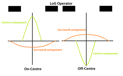
The difference in Gaussian model
In the visual cortex, elongated receptive fields for edge detection are formed by summing inputs from retinal ganglion cells. The simultaneous stimulation of the overlapping ON- and OFF- centre cells can therefore be explained by a zero-crossing (i.e. an edge).
The primal sketch is made up of disjointed edges, blobs, loops and bars, containing much less information than the retinal image, but featuring all of the important parts. The primal sketch forms the input for the second stage of processing, perceptual organisation. It is during perceptual organisation where larger regions and structures are formed by grouping parts of the image together. Furthermore, depth and motion are extracted from the retinal image and this forms the 2½D sketch, before becoming the 3D image.
The Marr-Hildreth Computational Model and Facial Recognition (Top)
The Marr-Hildreth model works very well in detecting edges, but in comparison to the efforts of an artist, it produces a very poor sketch of the human face. If the edges are all the same, then why is there a big difference? This hints that there must be additional processes that allow for perception of faces.
It also does not explain why we struggle with reversed contrast. If we are looking at the photonegative of a face, we as humans find it hard to recognise the face in contrast to the face in a normal image. If we relied on the edge-detection theory alone, then the edges should be identified in the same way and there should be no difficulty in identifying the face correctly.

If edges were the only feature in facial recognition, why are faces so hard to recognise when contrast is inversed? (Image/eyesonjason)
The poor face-recognition performance of the Marr-Hildreth model is thought to be due to faces having very a complicated 3D structure. The smoothing process changes features on faces enough that they do not produce these zero-crossings on the second derivative. Without the needed zero-crossings, identification of facial features using the Marr-Hildreth model is prevented. This means that, although a good model, it is far too simplistic to provide the complete answer for visual perception.
Other Routes to the Primal Sketch (Top)
The Marr-Hildreth model's edge detector theory is not the only way that the primal sketch can be created. Other mechanisms are thought to be in play and here are some of the other theories that supplement the edge-detectors idea, as well as may explain how we are able to perceive faces.
Valley Detectors
Valley detectors expand on the edge detector theory. These theoretical detectors can detect subtle changes in luminance over space and as such allow for more information to be taken from the retinal image to form the primal sketch.
Pearson and Robinson first described these valley detectors in 1985, which respond strongly to a peak-trough luminance profile. This allows for detection of lines and not edges. It is also worth noting that the valley detector has a similar composition to that of a cortical bar detector's receptive field, which further adds to the evidence of the existance of the valley detector (see the diagram on the right).
The investigators applied this valley-detecting filter to detect horizontal, vertical and diagonally orientated lines and found that this model provided a much better representation and preservation of detail to the relevant facial features that it was trying to detect.

The MIRAGE Model (Top)

The process involved in the MIRAGE model of vision and the final analysed sequence of Rs and Zs
The MIRAGE model utilises the LoG filters but does not focus on the zero crossings that they detect. Instead, it focuses on the sum of the positive values (S+) of the LoG filters used and all of the negative values (S-) used. The parts of the image where the S+ and S- form a zero are labelled as "Z" and parts of the image where there is a reponse are labelled as "R" (see diagram below). Edges, lines and areas of luminance all give different sequences of Rs and Zs to allow formation of a percept. As it stands, the MIRAGE model is a good representation of human vision.
Fourier Analysis (Top)
Another concept put forward is that of fourier analysis. This builds on from our knowledge that the information of different spatrial frequencies is carried through the visual system via different channels. Fourier analysis is the process of breaking the down these signals into multiple sine or cosine waves of varying spatial frequencies and amplitudes. It is thought that this process is used by our visual system on a localised scale
Further Reading (Top)
Additional information on these topics can be found via the following books (available on the Amazon Marketplace - purchase through these links will help support this website:
Algorithms for Image Processing and Computer Vision - by J.R. Parker
This book looks at the computerised models of how we see and can aid in understanding of the Marr-Hildreth model, edge-detectors and Laplacian of Gaussian operators.
Gaussian Scale-Space Theory - by Sporring, Nielsen, Florack and Johansen
Gaussian scale-space is one of the best understood multi-resolution techniques available to the computer vision and image analysis community. It covers the main theories associated with image analysis.
THIS CONCLUDES THE UNIT ON IMAGE ANALYSIS